Modeling 3D electromagnetic fields in complex geological structures

Electromagnetic modeling of large 3D geological structures with inhomogeneous background conductivity

Martin Čuma, Masashi Endo, Ken Yoshioka and Michael S. Zhdanov

Introduction

Geophysicists study propagation of physical fields through the earth's interior in order to determine its structure. The most common fields used are gravitational, magnetic, electromagnetic and seismic waves. Numerical modeling of known geological structure to produce geophysical field data represents forward problem. The goal of geophysical interpretation is to determine unknown geology by use of observed values of the geophysical fields. This is called an inverse problem. In practice, performing inversion involves minimization of misfit between observed field data and field data calculated by forward model based on structural properties inferred from the inversion. Thus, research in both forward and inverse modeling methods form an important part of geophysics.

Our group concentrates on use of electromagnetic (EM) methods, which study propagation of electric currents and electromagnetic fields through the earth. Here, the geological structure is usually characterized by its conductivity or resistivity. The basis of the electromagnetic fields theory is governed by Maxwell's equations, which equate electric field E and magnetic field H to conductivity σ, electric permittivity ε and magnetic permeability μ. The forward problem can be described by following operator equation:

{E,H} = A_em{σ,ε,μ}, (1)

where A_em is operator of the forward electromagnetic problem.

Similarly, inverse problem can be represented as

{σ,ε,μ} = (A_em)^-1{E,H}. (2)

Operator A_em is usually nonlinear. This leads to a set of integro-differential equations, which are solved in a discrete fashion on a 3D mesh.[1] In this article, we focus on recent progress with development of computationally efficient forward modeling methods.

Among the methods used to solve the forward problem we should mention Finite Elements (FE), Finite Difference (FD) and Integral Equation (IE) method. The IE method's main advantage over the former two is that one does not need to discretize the whole domain under study, but only usually much smaller domain of geological interest. The domain of interest is discretized on a 3D mesh with electromagnetic properties and fields calculated in each mesh cell. In the framework of the IE method, the conductivity distribution is divided into two parts: normal (background) conductivity σ_n and anomalous conductivity Δσ_a. Anomalous conductivity is considered only in the domain of interest, while normal conductivity is present throughout the whole model. The requirement for efficient method implementation using Green's functions necessitates use of horizontally homogeneous background. Fortunately, this situation is common as the anomaly of interest (ore deposit, hydrocarbon reservoir) is usually surrounded by layered uniform host rock.

EM survey typically consists of an array of receivers, which record earth response to EM signal transmitted by single or multiple transmitters, as seen in Figure 1. Solution of forward problem thus involves three distinct steps. First step calculates background fields induced on the receivers by the response of the homogeneous background. Second step calculates anomalous fields induced in the domain of interests. Finally, third step calculates fields on the receivers induced by the anomalous fields in the domain. The resulting field on the receivers is sum of the background field from step one and anomalous field from step three.

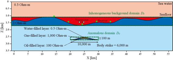
Figure 1. Vertical section model area with hydrocarbon reservoir and rough seafloor bathymetry. Survey receivers and transmitters are denoted with green and white dots, respectively. Sea water resistivity is 0.3 Ohm-m and subsurface background resistivity is 2 Ohm-m.

While the IE method is quite efficient compared to FE and FD, its main limitation is that its computational and memory requirements grow cubically with the increase of the domain dimension or with making the mesh finer (decreasing mesh cell size). Work on methods to alleviate this problem is ongoing. One of the recent contributions from our group is development of multi-grid (MG) approximation[2], which extrapolates electromagnetic fields on coarser grid (with larger cell size) to that on finer grid (with smaller, and thus more precise cell size).

In some applications, it is difficult to describe the geological model using horizontally layered background. As a result, the domain of interest may become too large for feasible calculation. We have recently developed a computational method that allows us to use variable background conductivity. In this article, we use this method, named Inhomogeneous Background Conductivity (IBC) method[3], to include the effect of underwater topography (bathymetry) in the EM field response. We use both explicit mesh and MG approximation to assess value of the MG method in the marine environment.

Integral equation solution using multigrid approach

As described in the introduction, we consider normal conductivity Δσ_n for the background and additional anomalous conductivity Δσ_a for the anomaly. For our discussion, we present derivations for the electric field E, similar equations can be obtained for magnetic field H. The integral representation of Maxwell's equations for total electric field E is

, (3)

where is the electric Green's tensor defined for an unbounded conductive medium with normal conductivity σ_n, G_E is corresponding Green's linear operator, and domain D corresponds to the volume within the anomalous domain with conductivity

, .

The total electric field can be also represented as a sum of background and anomalous fields:

. (4)

Multigrid approach is based on quasi-linear assumption that the anomalous field E^a is linearly proportional to background field Eⁿ through reflectivity tensor :

. (5)

Since the reflectivity tensor is linear, we can interpolate its value within the anomalous domain. We therefore solve the integral equation problem (3) on coarsely discretized grid Σ_c using complex generalized minimum residual method (CGMRM), obtaining background and anomalous fields at the coarse grid, Eⁿ(r_c) and E^a(r_c). We calculate reflectivity tensor on coarse grid as

,(6)

where i corresponds to x,y,z components and assuming that .

We then interpolate the reflectivity tensor to fine discretization grid Σ_f, and compute the anomalous electric field on the fine grid as

. (7)

We can now find the total electric field E(r_f) on the fine grid as

. (8)

Finally, using discrete analog of formula (3), we compute observed fields on the receivers.

Accounting for bathymetry with inhomogeneous background conductivity method

A topography structure is modeled as an inhomogeneous background domain B with conductivity σ_b = σ_n+Δσ_b; sum of horizontally layered (normal) conductivity σ_n and inhomogeneous conductivity Δσ_b. Consequently, Δσ_b within this domain generates field that induces additional field on the receivers and inside of the anomalous domain of interest A.

Total field at any point r_j is then expressed as a sum of normal field Eⁿ, variable background effect due to IBC Δσ_b and anomalous fields due to anomalous conductivity Δσ_a:

, (9)

where and are Green's linear operators for domain B and A, respectively.

Rewriting equation (9) for , we obtain equation for anomalous field in anomalous domain A:

(10).

In practice, we calculate field in domain B ignoring anomalous domain A, and use this field in equation (10) to obtain field in domain A. We then use equation (9) to get total field in the domain, and analog of equation (3) to calculate field at the receivers.

To improve accuracy, we can use this scheme iteratively. First iteration is performed as described above. Second iteration calculates field in domain B including the induction effect from anomalous field in domain A obtained at first iteration. The problem is then run until self consistency is reached for both anomalous fields and .

Application of IBC IE method to study bathymetry effects

We have incorporated the MG and IBC methods into our parallel forward modeling IE code called PIE3D. In this section, we present a practical case of modeling of marine controlled source electromagnetic (MCSEM) to evaluate feasibility of the MG and IBC methods for routine MCSEM use.

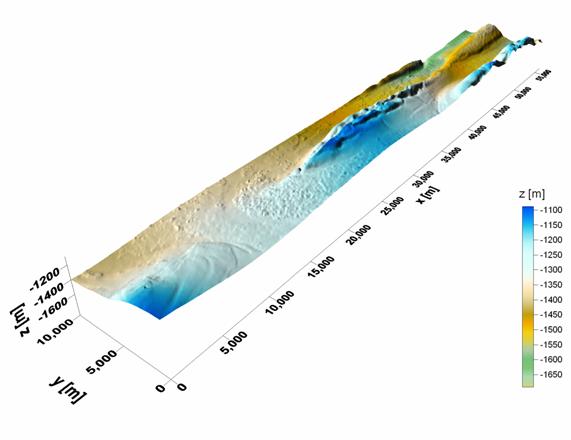
Sarawak Shell Berhad, Shell International Exploration and Production, and PETRONAS Managing Unit performed a bathymetry survey over geologically favorable target reservoirs in Sabah area in 2004. Relief of the bathymetry is depicted in Figure 2. The location of the hydrocarbon reservoir in this area has been estimated from seismic survey. We used the measured bathymetry data and positioned a synthetic reservoir-like geoelectrical structure to the same location where the actual reservoir has been found. The synthetic structure has a complex three dimensional geometry and contains three layers: a water-filled layer with a resistivity of 0.5 Ohm-m, a gas-filled layer with a resistivity of 1,000 Ohm-m, and an oil-filled layer with resistivity of 100 Ohm-m (Figure 3).

Figure 2. Bathymetry relief of the Sabah area.

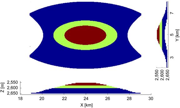
Figure 3. A model of a hydrocarbon reservoir located within the conductive sea-bottom sediment.

The EM fields in this model are generated by a horizontal electric dipole (HED) transmitter with a length 270 m and located at (x,y) = ( 24,5) km at a depth of 50 m above the sea-bottom. The transmitter generates the EM fields with a transmitting current of 1 A at 0.25 Hz. An array of sea floor electric receivers is located 5 m above the sea-bottom along a line with the coordinates ( x= 14,34} ,y=5 ) km with a spacing 0.2 km (Figure 1).

The survey area was represented by two modeling domains, D_a and D_b, outlined by the green dashed lines in Figure 1. Modeling domain D_b covers the area with conductivity variations associated with the bathymetry of the sea-bottom, while modeling domain D_a corresponds to the location of the hydrocarbon reservoir. We used 7,193,600 (1124 x 200 x 32) cells with each cell size 50 x 50 x 20 m for discretization of the bathymetry structure. The domain D_a of the hydrocarbon reservoir area was discretized by 1.5 million cells (400 x 240 x 16) with each cell size of 25 x 25 x 6 m to represent accurately the reservoir structure of the model.

Evaluating this model by any conventional IE method would require simultaneous solution of the corresponding system of equations on a grid formed by at least a combination of the two domains, D_a and D_b. Application of the IBC IE method allows us to separate the model into two subdomains, D_a and D_b. We solve the corresponding IE problem in these domains separately, which saves significant amount of computer memory and computational time. Moreover, we can save the precomputed Green’s tensors and fields, which includes the inhomogeneous background field, and reuse it in the iterative IBC approach, or for other computations with modified parameters of the reservoir. This brings about significant reduction of computational cost in the inverse problem solution during interpretation of practical EM field data.

To assess feasibility of the MG approach for bathymetry study, we ran one calculation using MG approximation. We also ran two explicit calculations, one fine grid discretization as detailed above, and other using coarse grid with twice the cell size (thus 8 times less cells) than the fine grid. The convergence plot of the iterative IBC modeling is shown in Figure 4 for fine grid and MG models and for both inhomogeneous background (bathymetry) and anomalous (reservoir) domains. The convergence rate is excellent. After just two iterations the relative errors in both bathymetry and anomalous domains are below the 10^-5 threshold. This is encouraging for prospective use in fast geological interpretation problems.

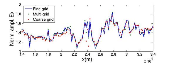
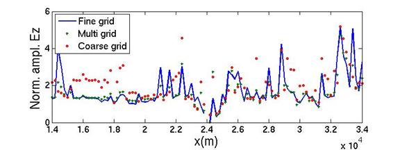
Figure 4. Convergence plot for the IBC modeling, red lines represent MG model, blue lines fine grid model; full line is anomalous domain D_a, dashed line bathymetry domain D_b

Figure 5. In-line (x direction) and vertical (z direction) electric fields along MCSEM profile.

Figure 5 shows total in-line and vertical electric field amplitudes along the MCSEM profile (y=5,000 m) at last IBC iteration normalized by the amplitude of the normal field. While the in-line (x direction) field values are very similar among the coarse, MG and fine grid, there are differences in the vertical (z direction) field. We attribute these differences to less detailed description of the bathymetry in case of the coarse grid, and to interpolation errors in the MG bathymetry domain field calculation. The coarse grid difference is substantial, while the MG matches the fine grid in most of the cases. While finer grid calculations can be expected to get the most precise results, time and resources savings using the MG approach warrant its applicability.

Computational requirements

The most computationally demanding part of the PIE3D code is calculation of anomalous electric field in the domains D_a and D_b. The limiting factor here is actually not as much the computation time, as the memory requirements to store the system of linear equations that describe the problem. In the fine grid calculation, for the larger bathymetry domain D_b, the required memory amounts 132 GB, for the smaller anomalous domain D_a, it equals 14 GB. Disk requirements for the intermediate data storage are also not negligible. Although the program uses efficient file compression algorithms, the total disk usage was about 400 GB. We have run the fine grid calculation on CHPC’s Delicatearch cluster, using 96 compute nodes, one processor per node. Each of the 96 processes used 1.5 GB RAM for the D_b field calculation. The smaller domain D_a required 48 CPUs. Total runtime of three IBC iterations was just over 3 hours.

In comparison, the MG calculation used just 24 nodes, 40 GB of disk space and needed about two hours to finish. Running on more nodes would probably not improve the performance significantly since the parallelization in current PIE3DMG code is limited to one domain dimension (z) and three field components. One of our future goals is to extend parallelizability to other dimensions and to transmitters and receivers. However, even it its current incarnation, MG provides viable alternative to fine grid modeling in case resources are scarcer or one needs to get the result faster.

Conclusions

In this research project, we have developed a parallel implementation of new integral equation (IE) method. This new method can improve the accuracy of the solution by iterative IBC calculation, and can reduce the computational cost by multi grid approach.

We have applied a new parallel code based on the IBC IE method for modeling the MCSEM data in the area with significant bathymetric inhomogeneities. Generally, this case requires large number of discretization cells to represent three-dimensional targets in the presence of the complex relief of the seafloor structure adequately. The IBC EM method allows us to separate this massive computational problem into at least two problems, which require considerably less resources.

Another advantage of the IBC IE method, which is more important in practical applications, is related to the fact that interpretation of the field data usually requires multiple solutions of the forward problem with different parameters of the target. The traditional computational method would require repeating these massive computations, including large number of cells covering the bathymetry, every time the model of the target is changed. On the other hand, using the IBC approach, we can pre-compute the bathymetry effect only once, and then repeat the computations on a smaller grid

covering the anomalous domain only. In addition, the multi grid approach can compute EM fields with even less computational cost without significant compromise in accuracy.

Acknowledgement

The authors acknowledge support of the University of Utah Consortium for Electromagnetic Modeling and Inversion (CEMI).

References