

|
|
|
Regularized Focusing Inversion
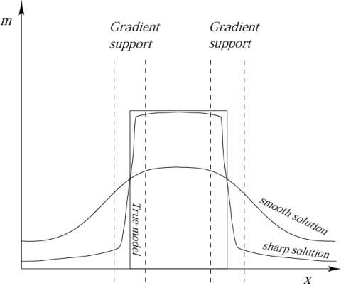
One of the critical problems in inversion of geophysical data is producing a stable solution, which at the same time can resolve complicated geological structures. We developed a new technique to solve this problem, which was called regularized focusing of inversion images. It is based on specially selected stabilizing functionals, which minimize the volume of the anomalous zone and/or the area where strong model parameter variations and discontinuity occur. The main application of the stabilizing functionals (the stabilizers) is in bringing the a priori information about the desirable properties of the solution into the inversion algorithm. Traditional inversion is based on the "maximum smoothness" stabilizing functionals. This approach does not allow detecting sharp boundaries between different geological formations. In mineral exploration, it is useful to search for a stable solution within the class of inverse models with sharp geological boundaries. Figure 1 shows, for example, an application of the minimum gradient support functional to recover the sharp boundary of the one- dimensional structure.
We have demonstrated that focusing inversion could generate more focused and clear images for geological structures than regularization based on conventional maximum smoothness criteria (see, for example, the recent text on inversion theory: Zhdanov, M.S., 2002, Geophysical Inverse Theory and Regularization Problems, Methods in Geochemistry and Geophysics, 36, Elsevier, 628 pages, ISBN: 0-444-510893. http://www.elsevier.nl/inca/publications/store/6/2/2/7/2/6/index.htt).
We believe that the application of focusing to inversion can bring a breakthrough in the solution of the geophysical 3-D inverse problems. We apply this technique now to 3-D gravity, 3-D magnetic, and 3D gravity gradiometer data inversion. Our inversion method is designed for inversion of the anomalous gravity and/or any component of the anomalous magnetic field, including a total magnetic anomaly. Recently we developed also a method and a computer code for 3-D tensor gravity field inversion, based on ideas of data compression and image focusing.
Illustration of the effectiveness of the focusing inversion using magnetic field example (after Portniaguine and Zhdanov, 2002)
As an example, we present here a comparison between smooth inversion and focusing inversion results for 3-D interpretation of magnetic data (Portniaguine and Zhdanov, 2002). Figures 2 and 3 show the models used for inversion and the corresponding maps of the observed magnetic field. Figures 2-5 present the true models and the inversion results obtained by the smooth inversion and focusing inversion respectively. Note that the smooth inversion generates a slightly diffused image of the models, while the focusing inversion generates clear and sharp images.
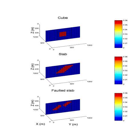
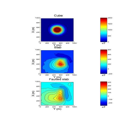
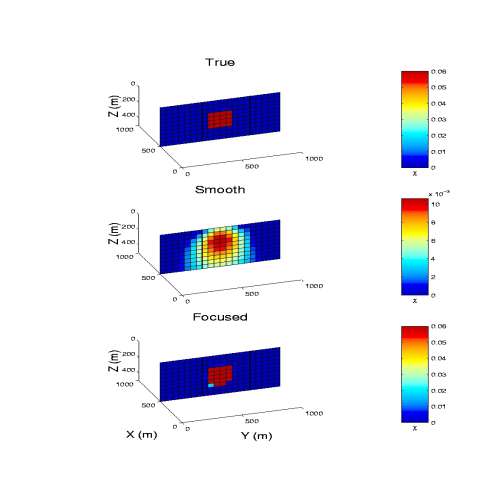
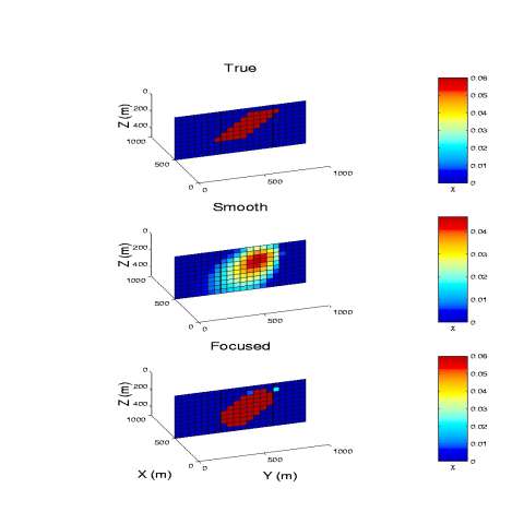
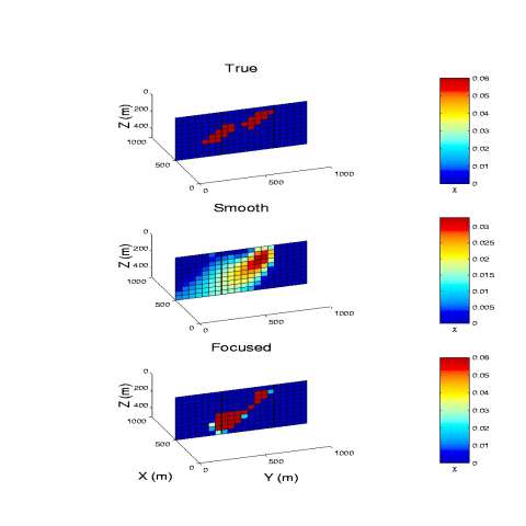
Illustration of the effectiveness of the focusing inversion using cross-well tomography example (after Zhdanov and Yoshioka, 2003).
We use similar ideas in the new generations of CEMI
3-D EM inversion codes that can be used for interpretation of 3-D
MT, CSMT, and TDEM data, including surface to borehole, and
borehole configurations. As an example we will present below a
comparison between smooth inversion and focusing inversion results
for 3-D cross-well electromagnetic tomography. We generated the
synthetic EM data for a geoelectrical model of a dipping
conductive body with the resistivity 10 Ohm-m in a 100 Ohm-m
homogeneous background (Figure 7). The electromagnetic field in
the model is generated by a vertical magnetic dipole transmitter
moving vertically along the left and right boreholes and
transmitting a signal every 10 meters. The tri-axial magnetic
component receivers are located along both boreholes deployed in
the ![]() -direction with
10 m separation.
-direction with
10 m separation.![]() The
synthetic data for this model for four frequencies, 10, 30, 100,
and 300 Hz, were computed using the integral equation forward
modeling code SYSEM (Xiong, 1992). The data were contaminated by
2% Gaussian noise and inverted using smooth and focusing
regularized inversion. The area between two boreholes, used for
inversion, was divided into 896 cells (8
The
synthetic data for this model for four frequencies, 10, 30, 100,
and 300 Hz, were computed using the integral equation forward
modeling code SYSEM (Xiong, 1992). The data were contaminated by
2% Gaussian noise and inverted using smooth and focusing
regularized inversion. The area between two boreholes, used for
inversion, was divided into 896 cells (8 ![]() 8
8 ![]() 14 cells in
14 cells in ![]() directions), with the size of cells 10 x 10 x 10 m
directions), with the size of cells 10 x 10 x 10 m![]() .
.
Note that in order to generate a good quality
synthetic data, we used finer discretization for forward modeling
than for inversion. In particular, in forward modeling the
conductive body was divided into 25 cells (5 ![]() 5
5 ![]() 5 cells in
5 cells in ![]() directions), with the
size of cells 5 x 5 x 5 m
directions), with the
size of cells 5 x 5 x 5 m![]() .
.
Figure 8 presents the results of the traditional smooth inversion with the minimum norm stabilizing functional (Zhdanov, 2002) for a model of the conductive dipping dike. We can see the location of the targets in this image; however, the resistivity is significantly smoothed and overestimated. Figures 9 and 10 show the results of the focusing inversion for the same model. One can see that the image is sharp and bright, and the shape and location of the target is reconstructed very well.
These examples illustrate the practical efficiency of the regularized focusing inversion in geophysical imaging of the underground formations.
All CEMI inversion codes are equipped with the options to run the smooth or focusing inversion. The users may select the appropriate solution depending on the a priori information about the geological target.
References
Portniaguine O., and M. S. Zhdanov, 2002, 3-D magnetic inversion with data compression and image focusing: Geophysics, 67, No. 5, 1532-1541.
Xiong, Z., 1992, EM modeling of three-dimensional structures by the method of system iteration using integral equations: Geophysics, 57, 1556-1561.
Zhdanov, M. S. 2002, Geophysical inverse theory and regularization problems: Elsevier, Amsterdam - New York - Tokyo, 628 pp.
Zhdanov, M. S. and K. Yoshioka, 2003, Cross-well electromagnetic imaging in three dimensions: Exploration Geophysics, in publication.