

|
|
|
3-D interpretation of the induced polarization data based on the complex conductivity relaxation models
By Ken Yoshioka and Michael S. Zhdanov
The quantitative interpretation of IP data in a complex 3-D environment is a very challenging problem. The analysis of IP phenomena is usually based on models with frequency dependent complex conductivity distribution. One of the most popular is the Cole-Cole relaxation model and its different modifications. The parameters of the conductivity relaxation model can be used for discrimination of the different types of rock formations, which is an important goal in mineral exploration.
We have developed recently a technique for detecting the IP effects in frequency domain and time domain electromagnetic (EM) data and three-dimensional inversion of this data based on the appropriate relaxation models. This method takes into account the nonlinear nature of both electromagnetic induction and IP phenomena and inverts the EM data for the relaxation model parameters (Yoshioka and Zhdanov, 2003).
Numerical modeling results
We will illustrate the outlined above approach to IP
data inversion using numerical simulation. We have generated the
synthetic EM data for the typical geoelectrical models of the
conductive or resistive targets within a homogeneous background.
As an example, we will present the results of the numerical
simulation for just one geoelectrical model shown in Figure 1. The
electromagnetic field in the model is generated by electric bipole
transmitters with a length of ![]() m (galvanic EM field excitation) and is measured by
electric bipole receivers of the same length. The transmitters and
receivers are positioned along a set of profiles deployed in the
m (galvanic EM field excitation) and is measured by
electric bipole receivers of the same length. The transmitters and
receivers are positioned along a set of profiles deployed in the ![]() -direction with 50 m
separation (Figure 1, top section). A geoelectrical model
represents two conductive bodies in a 100 Ohm-m homogeneous
background with the same resistivity and chargeability, but with
the different values of the time parameter
-direction with 50 m
separation (Figure 1, top section). A geoelectrical model
represents two conductive bodies in a 100 Ohm-m homogeneous
background with the same resistivity and chargeability, but with
the different values of the time parameter ![]() and the relaxation parameter C (Figure
1, bottom section). The Cole-Cole model parameters for each body
are defined according to Table 1 (the left body has the parameters
corresponding to Cole-Cole model 1, while the write body has the
parameters of the Cole-Cole model 2):
and the relaxation parameter C (Figure
1, bottom section). The Cole-Cole model parameters for each body
are defined according to Table 1 (the left body has the parameters
corresponding to Cole-Cole model 1, while the write body has the
parameters of the Cole-Cole model 2):
Table 1
The synthetic EM data for this model were generated using integral equation forward modeling code SYSEM (Xiong, 1992) for a frequency range from 0.125 to 64 Hz. The synthetic observed data were contaminated by 2% Gaussian noise and inverted using focusing regularized inversion (Yoshioka and Zhdanov, 2003).
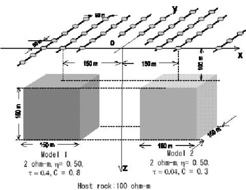
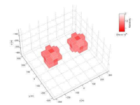
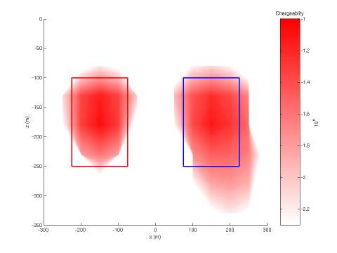
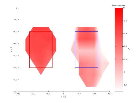
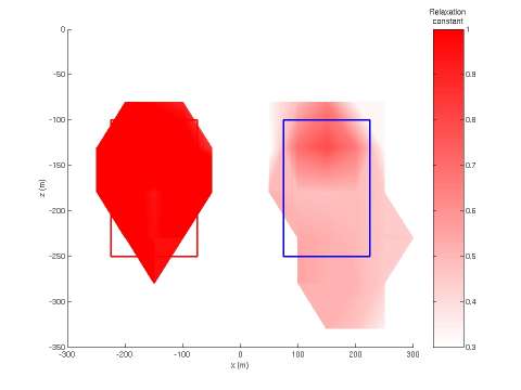
Figure 2 presents a 3-D image of the result of the inversion for the DC resistivity. Figure 3 shows the same vertical cross-section of the recovered chargeability over the line passing above the centers of two bodies. The vertical cross-sections of the distribution of the time parameter, t and the relaxation parameter C are shown in Figures 4 and 5 respectively. One can see that the inversion produces good images of the spatial distribution for all different relaxation model parameters: resistivity, chargeability, time and relaxation parameters. Using these images, one can reconstruct the location of the bodies from the resistivity and chargeability images, and evaluate additional Cole-Cole model parameters from the time and the relaxation parameter images. These parameters may be used for the discrimination of the different rock formations, which is an important goal in mineral exploration. One application, for example, will be sulfide mineral discrimination with the multi-frequency IP.
REFERENCES
Yoshioka, K., and M. S. Zhdanov, 2003, Nonlinear regularized inversion of array induced polarization data based on the Cole-Cole model: Proceedings of 2003 CEMI Annual Meeting, 201-224.