

|
|
|
Fast 3-D inversion of the controlled source electromagnetic data
By Michael S. Zhdanov and Gabor Hursán
In this project we address one of the most challenging problems of electromagnetic (EM) geophysical methods: 3-D inversion of the controlled source EM data over inhomogeneous geological formations. The difficulties in the solution of this problem are two-fold. 3-D EM forward modeling is an extremely complicated and time-consuming mathematical problem itself. Moreover, the inversion is an unstable and ambiguous problem. To overcome these difficulties in the initial stage of iterative inversion, we apply for forward modeling the quasi-analytical (QA) approximation developed recently by Zhdanov et al. (1999, 2000). In the final stage of the iterative inversion we use the Contraction Integral Equation method of the rigorous forward modeling (Hursán and Zhdanov, 2002).
To obtain a stable solution of a 3-D inverse problem we apply the regularization method based on using a focusing stabilizing functionals (Portniaguine and Zhdanov, 1999; Hursan and Zhdanov, 2000; Zhdanov, 2002). These stabilizers help to generate a sharp and focused image of anomalous conductivity distribution. The developed algorithm is implemented in the computer code QAINV3D. The new recently released version of this code can run 3-D inversion of both the controlled source EM data (CSEM) and of the magnetotelluric (MY) data. In the CSEM case, many different sources of EM field can be used: electrical and magnetic dipole with different orientations, circular and rectangular transmitter loops, electrical bipoles of arbitrary lengths, etc. The code can process the different components of the observed electric and/or magnetic fields, and the MT impedances as well. The output of the inversion consists of the volume distribution of the anomalous conductivity on the given rectangular grid. The size of the grid is limited only by the computer memory available. In our practice we have experimented with the grid consisting of up to 50,000 cells. The computational time for inversion, typically, does not exceed thirty minutes on 1 GHz PC. We present a few examples of the CSEM data inversion using QAINV3D code.
Model studies
Model 1
Model 1 consists of a homogeneous half-space with resistivity of 100 Ohm-m, containing a conductive tilted dyke structure with the resistivity of 16 Ohm-m (Figure 1).
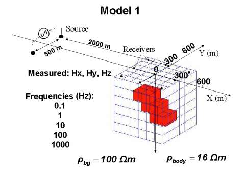
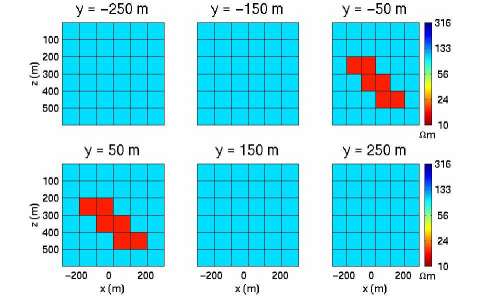
This model is excited by an electric current bipole with 500 meters electrode separation. The source is located 2000 meters from the center of the inhomogeneity. The source has been fed by alternating currents with five different frequencies: 0.1, 1, 10, 100 and 1000 Hz. The x, y and z components of the anomalous magnetic field have been simulated at nine receiver points arranged on a homogeneous grid. The inverted area is a homogeneous mesh consisting of 6 X 6 X 6 cubic cells surrounding the anomalous structure to be inverted. The vertical slices of the inverted area and the true model are presented in Figure 2.
The data vector consists of 135 simulated field components. The synthetic data is generated by a full integral equation code and it has been contaminated by 3 percent random noise. The model parameters are the unknown anomalous conductivity values of each cell of the inverted area. The inversion problem is ill posed and underdetermined, so we used the regularized conjugate gradient method. We performed quasi- analytical (QA) inversion with focusing stabilizer. The results of QA inversions are shown in Figure 3.
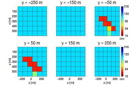
We obtain an image, which corresponds well to the true model. The difference between the synthetic data computed by QA approximation and full IE solution is less than the given noise level.
Model 2
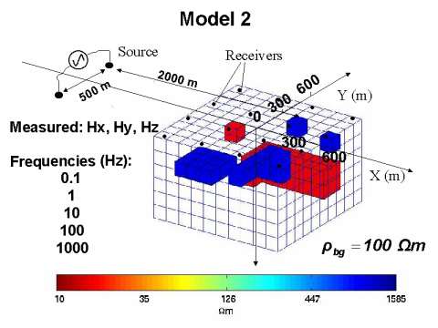
Model 2 represents a more complicated structure with several resistive and conductive bodies. The background model and the source are exactly the same as in Model 1. The frequencies were 0.1, 1, 10, 100 and 1000 Hz. In this experiment, like in Model 1, we simulated the three components of the anomalous magnetic field by solving a full IE, and the data has been contaminated by 3 percent random noise. The receivers are located on a 4 X 4 grid at the surface (z = 0). The inverted area has been discretized by 10 X 10 X 6 cubic cells of 100 m size in the x, y and z directions.
The 3-D picture of the model and the measurement system with the inverted area is presented in Figure 4. Figure 5 provides horizontal slices giving a more detailed image of the model.
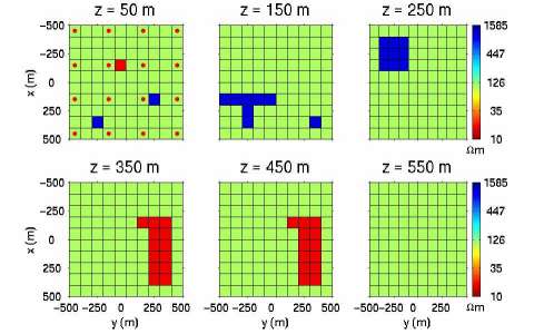
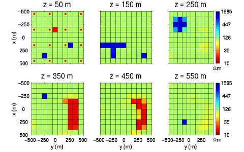
Similarly to the previous model study, we performed focusing QA inversion (Figure 6). We can see that even such a complicated 3-D model can be reconstructed based on a relatively small amount of data.
The future directions for research will include extending this method and computer code for the inversion of the time domain EM data.
References
Hursán, G. and M. S. Zhdanov, 2002, Contraction integral equation method in 3-D electromagnetic modeling: Radio Science, 37, No. 6, 1089.
Portniaguine O., and M. S. Zhdanov, 1999, Focusing geophysical inversion images: Geophysics, 64, No. 3, 874-887.
Zhdanov, M. S., Dmitriev, V. I., Fang, S., and G. Hursán, 1999, Quasi-analyticalapproximations and series in 3-D electromagnetic modeling: Proceedings of the Second International Symposium on three-dimensional electromagnetics, University of Utah, Oct. 16-20, 1999.
Zhdanov, M. S., Dmitriev, V,I,. Fang, Sh., and G. Hursán, 2000, Quasi-analytical approximation and series in 3D electromagnetic modeling: Geophysics, 65, 1746-1757.
Zhdanov, M. S. and G. Hursán, 2000, 3-D electromagnetic inversion based on quasi-analytical approximation: Inverse Problems, 16, 1297-1322.
Zhdanov, M. S. 2002, Geophysical inverse theory and regularization problems: Elsevier, Amsterdam - New York - Tokyo, 628 pp.